This study involved 39 patients with several liver diseases and after obtaining written informed consent,
all patients underwent an MR examination including conventional MRE and diffusion-weighted image (DWI) sequence (see Table 1).
In the DWI sequence,
27 patients and 12 patients were scanned using 3 and 5 b-value,
respectively.
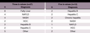
Table 1
MR imaging
1.
MRE protocol
An external driver device (60 Hz) was used to induce shear waves in the liver tissue,
and axial imaging of the abdomen with breath-holding was performed for conventional MRE.
Imaging parameters were repetition time (TR),
33.3 ms; echo time (TE),
22.1 ms; flip angle,
30 degrees; field of view,
256 × 256; matrix size,
256 × 256; and slice thickness,
8 mm.
Next,
shear stiffness maps were generated using a multi-scale direct inversion algorithm on the MRI equipment.
2.
DWI protocol
In addition,
DWI with a fat-suppressed spin-echo echo-planar sequence was performed with the following parameters (see Table 2): TR,
12000 ms; TE,
89 ms; flip angle 30 degrees; matrix size,
256 × 256; slice thickness,
5 mm; and b-values,
0,
50,
200,
800,
and 1500 s/mm2.
For b-value,
data acquisition was performed separately for each three (0,
200,
and 1500 s/mm2) and five b-value (0,
50,
200,
800,
and 1500 s/mm2).
For the patient DWIs acquired with the three and the five b-values,
a number of excitations (NEX) were applied to each b-value to improve the signal-to-noise ratio (SNR) of the DWI.
In three b-value,
one,
two,
and four of NEX were selected as 0,
200,
and 1500 s/mm2,
respectively.
In five b-values,
one of NEX value was selected at 0-800 s/mm2 of the b-values,
and three NEX values were used at only 1500 s/mm2 of the b-value.
Here,
all imaging parameters and setting value are shown in Table 2.
Data processing
In this study,
Vitrea® software (Canon Medical Systems Corporation,
Tochigi,
Japan) and in-house software were used to generate several calculated maps (Matlab R2015b; MathWorks).
The illustration of procedure of the experiments are shown in Figure 1.
Shear stiffness of tissues of each of the patients was calculated from the conventional MRE data (see Figure 1a).
Two ADC maps,
which have different diffusion components,
such as fast and slow diffusion components,
were calculated from a slope of the DW signal attenuation between two b‒values (ADC0‒200 s/mm2,
ADC200‒1500 s/mm2) for each three and five b-value.
Moreover,
ADC0-1500 s/mm2,
D,
D*,
and α map were calculated from fitted signal attenuation curves with mono‒exponential,
bi‒exponential,
and stretched‒exponential models using Bayesian fitting algorithms (see Figure 1b).
All estimated parameter maps are represented as follows:
1.
Two ADC maps derived from the slow and fast diffusion components without the non-least square method.
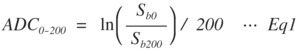
Fig. 1: Eq.1
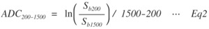
Fig. 2: Eq.2
where S is the DW signal and subscripts b0-b1500 indicate b-values.
In particular,
ADC200-1500 is more sensitive than ADC0-200 with respect to the shear elasticity of the biomaterials [5].
2.
The estimated parameter maps for each of the IVIM models with non-least square method using the Bayesian fitting algorithm.
a.
mono-exponential
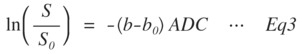
Fig. 3: Eq3
b.
bi-exponential
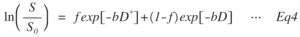
Fig. 4: Eq.4
c.
stretched exponential
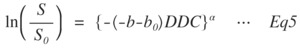
Fig. 5: Eq.5
where,
the b and b0 are the b-values of the desired value and 0 s/mm2.
In this study,
0,
50,
200,
800,
and 1500 s/mm2 of the b-values were used.
An illustration of experimental procedure is shown in Figure 1.
Data statistics
A region of interest (ROI) analysis was performed for each patient and was placed on the liver of α map avoiding unwanted signals,
such as a large vessel region for each three and five b-value (see Figure 1c).
In this study,
threshold values were applied to each of the estimated parameters to remove the component of inhomogeneous signal variance caused by the vessels,
low SNR,
and other imperfections in the liver,
as shown in Figure 1d.
For the α map,
the threshold values were determined from α (0.01 < α < 1).
ADC0-200 and ADC200-1500,
a threshold of less than 0.025 mm2/s was then used to remove unwanted ADC signals.
No threshold was used for the D* and D values in this study.
After removing unwanted signals in the ROI,
linear regression for each of the patients was applied to the conventional shear stiffness against the estimated parameter map of the IVIM model on the ROI.
Outliers of the mean value were systematically excluded for each of the linear regression results (see Figure 1e).
Finally,
the IVIM maps were empirically converted to virtual shear stiffness from the results of linear regression with the removed the outliers (see Figure 1f).
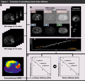
Fig. 6
