A homogeneous spherical phantom filled with a paramagnetic solution (NiSO4) and 10 healthy subjects were scanned with a 3T MAGNETOM Skyra system (Siemens Healthcare,
Erlangen,
Germany) and a 64-channel head coil,
using the same acquisition protocol which is detailed in Table 1.
|
TABLE 1: ACQUISITION PARAMETERS
|
| |
WB VIBE |
VIBE |
B1 MAP |
GRAPPATINI |
3D MPRAGE |
| FOV (mm) |
230*230 |
230*230 |
230*230 |
230*216 |
230*230 |
|
VOXEL SIZE
(mm)
|
1.8*1.8*3 |
1.8*1.8*3 |
1.8*1.8*7.5 |
1.2*1.2*4 |
0.9*0.9*0.9 |
| TR (ms) /TE(ms) |
5.45/1.46 |
5.45/1.46 |
10390/1.9 |
5420 /10.1 TO 161.1 (16 ECHOES) |
2400/2 |
| FLIP ANGLE (deg) |
30 |
2-3-5-8-10-12-15-18-25-30 |
8 |
180 |
8 |
|
SLICE N./
THICK(mm)/
GAP(mm)
|
52/3/0.6 |
18/3/0.6 |
6/7.5/1.5 |
32/4/0.4 |
224/0.9/0 |
| GRAPPA FACTOR |
2 |
2 |
// |
2 |
2 |
|
ACQUISITION TIME
(min:s)
|
02:14 |
00:45*10 |
02:05 |
01:44 |
05:45 |
|
MARTINI ACCEL.
FACTOR
(BLOCK SCHEME)
|
// |
// |
// |
5 |
// |
|
AVERAGES
|
6 |
6 |
1 |
1 |
1 |
T2 maps: for fast T2 mapping,
a multi-spin-echo acquisition with a highly accelerated k-space sampling was used.
This prototype sequence dubbed GRAPPATINI [3] combines a model-based MARTINI [4] approach with parallel imaging and provides an online calculation of T2 maps.
The k-space is split into five blocks,
only one block being measured at each echo time with a rotating scheme and for a total of 16 echoes (central blocks are oversampled).
Moreover,
each block is also undersampled with a GRAPPA 2 approach,
alternating non-sampled lines at each block.
T2 maps were calculated inline on the scanner using the mono-exponential model-based iterative GRAPPATINI algorithm.
In order to further reduce scan time (1’44’’),
a slice thickness of 4 mm with a 1 mm gap was chosen.
The ten subjects centre slice volume positions were averaged and used as a reference for phantom positioning.
An example of T2 map is shown in Fig.1
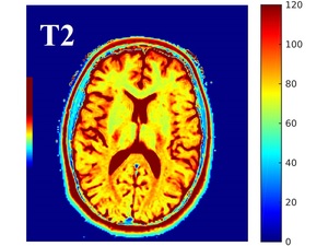
Fig. 1: Example of T2 map output
T1 maps: for T1 mapping,
ten RF-spoiled 3D gradient echoes (VIBE) acquisitions were obtained,
with flip angles from 2° to 30° and a reduced scan volume to cover GP in the shortest possible time (45’’ for each acquisition).
Two fast acquisitions with different TEs for B1 map calculation,
which was processed online,
were used to correct VIBEs nominal flip angles.
An extra 30° VIBE covering the whole brain (WB-VIBE) was added for post-processing purposes.
The phantom volume centring strategy was the same as described for T2 maps.
T1 maps were calculated offline with a Matlab script (The MathWorks,
Inc.,
Natick,
Massachusetts,
United States) using a model-based non-linear fit.
R2 maps were also output for visual assessment of goodness of fit.
An example of T1 and R2 maps is shown in Fig.
2 and Fig.3.
For co-registration purposes,
whole-brain maps covering the same WB-VIBE volume were calculated (WB-T1),
adding some fake slices to the original volume with a zero-padding operation.
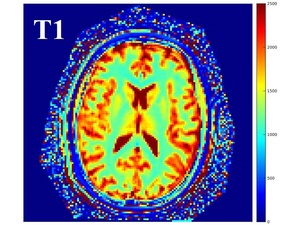
Fig. 2: Example of T1 map output
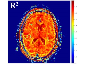
Fig. 3: Example of R2 map output
For GP segmentation,
a T1-weighted gradient echo (3D-MPRAGE) scan covering the whole brain was obtained.
In-vivo image processing: a flow chart of the entire processing for T1 evaluations is shown in Fig.
4.
In order to analyse GP-T1 and GP-T2 statistics,
an automated GP segmentation of the MP-RAGE was carried out with FSL FIRST[5] and the output mask was further 3D-eroded by 1 pixel to reduce possible partial volume effects (OUT-MASK).
T2 maps were aligned to the 3D-MPRAGE with an affine registration performed with FSL FLIRT[6,7].
The quality of the alignment was checked by an experienced Neuroradiologist (15 yrs).
The OUT-MASK was used as a filter to extract GP-T2 distributions from the co-registered map.
For T1,
the processing comprised a WB-VIBE registration to the 3D-MPRAGE and the application of the transformation matrix to the WB-T1.
The resulting registered WB-T1 was then filtered with the OUT-MASK for GP-T1 statistical analysis.
Left and right globus pallidi were separately investigated.
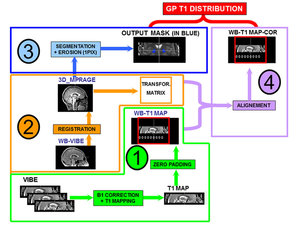
Fig. 4: Processing flowchart for globus pallidus T1 calculation
Phantom image processing: for each subject,
the two transformation matrices from T1 and T2 registration processing were used to align the phantom T1 and T2 maps to the subject 3D-MPRAGE.
The ‘PHANTOM’ GP-T1 and ‘PHANTOM’ GP-T2 distribution analysis were performed with the same OUT MASK filtering process used for in-vivo measurements.
Additionally,
the variability of relaxation times was investigated in a region of interest about 80% of phantom image volume,
for a global uniformity reference.
The spatial variability is defined by the variation coefficient of the relaxation times within the segmented ROIs.
Note that the lower is the spatial variability the higher is the uniformity.
Statistical analysis of the T1 and T2 distributions was carried out with Statgraphic Centurion XV (Statgraphic Technologies Inc.,
The Plains,
Virginia)
