ECR 2014 / C-1010
Dynamic High resolution Sonography (d-HRUS) of lower limb muscles: a detailed didactic approach
This poster is published under an open license. Please read the disclaimer for further details.
Congress:
ECR 2014
Poster Number:
C-1010
Type:
Educational Exhibit
Keywords:
Musculoskeletal system, Ultrasound, Education, Athletic injuries, Education and training
Authors:
S. Perugin Bernardi1, A. Corazza2, D. Orlandi2, R. Sartoris2, G. Ferrero2, E. Silvestri2; 1Genova/IT, 2Genoa/IT
DOI:
10.1594/ecr2014/C-1010

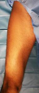
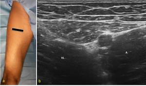
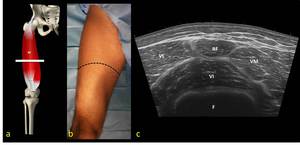
Fig. 1:
Lower limb position to evaluate the anterior thigh compartment.
 and sartorius muscle (SA).")
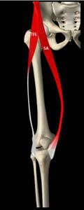
Fig. 2:
Anatomical scheme of tensor muscle of fascia lata (TFL) and sartorius muscle...
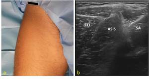
 Probe position to evaluate the proximal insertion of sartorius (SA) and tensor Fasciae Latae (TFL) muscles at ASIS (anterior-superior iliac spine) level. (b) US axial scan : note the typical “pseudo-thyroid” aspect of insertions of tensor muscle of fascia lata (TFL) and sartorius (SA) muscle on ASIS.")
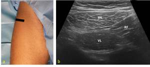
Fig. 3:
(a) Probe position to evaluate the proximal insertion of sartorius (SA) and...
 Probe position to evaluate tensor of fascia lata (TFL) at proximal third of the thigh on axial plane ; (b) US axial scan at proximal lateral third of thigh illustrates the relationship among the TFL and the vastus lateralis (VL) and rectus femoris (RF) muscles.")
Fig. 4:
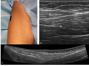
(a) Probe position to evaluate tensor of fascia lata (TFL) at proximal third of...
Probe position to study TFL on longitudinal scan;(b)Longitudinal US scan : distal insertion of TFL muscle on anterior aspect of fascia lata (FL) that appears as a hyperechoic cordon like band. Vastus lateralis muscle (VL) is deeper than TFL; (c)Extended field of view (EFV) US longitudinal scan of TFL muscle from proximal to distal insertion.")
Fig. 5:
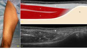
(a)Probe position to study TFL on longitudinal scan;(b)Longitudinal US scan :...
 Probe path to evaluate the ileotibial tract on the longitudinal plane;(b) anatomical scheme of ileotibial tract(*);(c) EFV US longitudinal scan of ileotibial tract to the lateral femoral condyle. Ileotibial tract appears like a fibrillar structure located superficially than vastus lateralis (VL) and vasutus intermedius (VI) muscles.")
Fig. 6:
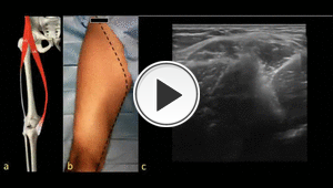
(a) Probe path to evaluate the ileotibial tract on the longitudinal plane;(b)...
 Probe position to evaluate the sartorius muscle (SA) at the proximal third of thigh on the axial plane; (b) US axial scan: in the proximal third of thigh SA is in a superficial position, under the fascia and near the femoral vascular bundle. VL; vastus lateralis muscle; A, adductor lungus muscle.")
Fig. 8:
(a) Probe position to evaluate the sartorius muscle (SA) at the proximal third...
 lies deep to the RF.")
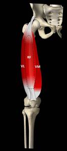
Fig. 9:
Anatomical scheme of quadriceps muscle group: RF, rectus femoris; VM, vastus...
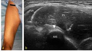
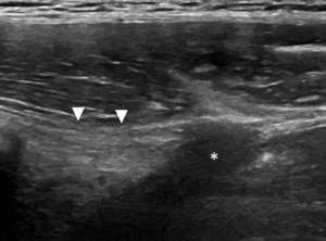
 Probe position to visualize RF muscle proximal insertion on anterior-inferior iliac spine (AIIS) on the axial plane. (b) US axial scan at AIIS level shows the proximal insertion of the RF muscle. The tendon has an ovular hyperechoic appearance (arrowhead) just under the psoas muscle (PS). SA, sartorius muscle.")
Fig. 10:
(a) Probe position to visualize RF muscle proximal insertion on...
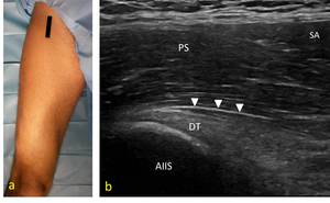
 Probe position to evaluate the direct tendon (DT) of the RF muscle on the longitudinal plane. (b) US longitudinal scan of the direct tendon insertion (arrowheads) into the AIIS (anterior-inferior iliac spine). PS, psoas muscle; SA, sartorius.")
Fig. 11:
(a) Probe position to evaluate the direct tendon (DT) of the RF muscle on the...
 and indirect (*) tendon of the RF muscle. Identify the hypoechoic appearance of the indirect tendon caused by the change in orientation of its fibres (anisotropy), which runs obliquely and externally compared to the direct tendon.")
Fig. 12:
US longitudinal scan shows the direct (arrowheads) and indirect (*) tendon of...
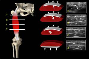
 correlated to EFV US axial scan(c) at middle third of the thigh(b) that shows the anatomical relationship among the vastus intermedius (VI), vastus medialis (VM), vastus lateralis (VL) and rectus femoris (RF) muscles.")
Fig. 13:
Anatomical scheme(a) correlated to EFV US axial scan(c) at middle third of the...
 Proximal third of the RF muscle. Visualize the superficial aponeurosis (arrowheads), just under the sartorius (SA) and the central aponeurosis (*).
(b,b’) (c,c’) Proximal and distal middle third of the RF muscle. Note the typical “comma-shaped” appearance of the central aponeurosis (*).
(d,d’) Distal third of the RF muscle. The deep aponeurosis (arrow) is seen as a hyperechoic band between the RF muscle and the VI muscle.")
Fig. 14:
Anatomical schemes correlated to US axial scans at different levels of the RF...

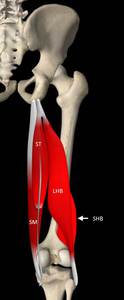
Fig. 16:
Anatomical scheme of posterior thigh compartment muscles : SM, semimembranosus;...
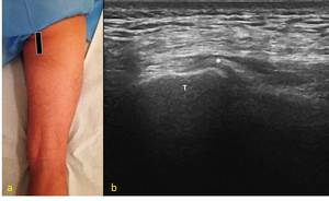
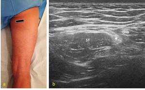
 Probe position to evaluate the hamstrings’insertion (*) into the ischiatic tuberosity on the longitudinal plane. (b) US longitudinal scan : note the conjoined insertion on ischiatic tuberosity (T) of semimebranosus, semitendinosus and long head of biceps femoris.")
Fig. 17:
(a) Probe position to evaluate the hamstrings’insertion (*) into the...
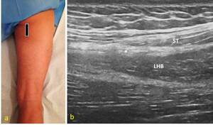
 Probe position to evaluate the common tendon (*) of the semitendinosus (ST) and long head of biceps femoris (LHB) muscles on the longitudinal plane. (b) US longitudinal scan of the common tendon with a hyperechoic fibrillar apparence.")
Fig. 18:
(a) Probe position to evaluate the common tendon (*) of the semitendinosus (ST)...
 Probe position to evaluate the common tendon (*) of the semitendinosus (ST) and long head of biceps femoris (LHB) muscles on the axial plane. (b) US axial scan : note the hyperechoic “comma-shaped” appearance of the common tendon.")
Fig. 19:
(a) Probe position to evaluate the common tendon (*) of the semitendinosus (ST)...
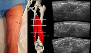
 Proximal third. EFV axial scan visualizes the large aponeurosis of semimembransus (SM) which continues in the proximal tendon. Aponeurosis presents a hyperechoic aspect between the semitendinosus (ST) and the aductor magnus (AM) muscles; ST lies just lateral to SM; long head of biceps femoris (LHB) is the most lateral ischiocrural muscles. (b, b’) Middle third. EFV axial scan shows SM with a triangular shape medial to ST. Note the internal septum of ST that appears like a fibrillar hyperechoic band within the muscle belly. LHB has an organized internal structure.(c, c’) Distal third. EFV demonstrates the SM lateral to sartorius muscle (SA), the myotendinous junction of ST with the eccentric distal tendon superficial to SM belly. At this level short head of bicep femoris (SHB) is separated to LHB by a distal aponeurosis which is seen as an hyperechoic band .")
Fig. 20:
Anatomical scheme correlated to EFV US axial scans at different levels of the...

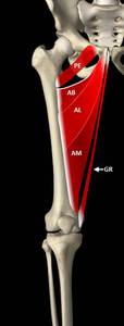
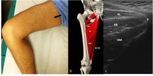
Fig. 22:
Anatomical scheme of medial thigh compartment muscles : PE, pectineus; AB...
 Probe position to evaluate the proximal insertion of adductor muscles in the anterior surface of the pubis on the sagittal plane. (b) Anatomical scheme of medial thig compartment musclse.PE, pectineus; AB, adductor brevis; AL, adductor longus; AM, adductor magnus; GR, gracilis. (c) US sagittal scan : note the three muscle layers represented from superficial to deepest by AL,AB and AM.")
Fig. 23:
(a) Probe position to evaluate the proximal insertion of adductor muscles in...

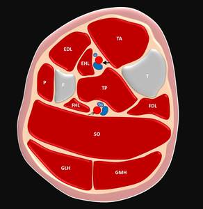
Fig. 26:
Cross sectional anatomical scheme of leg at middle third level. TA, tibialis...
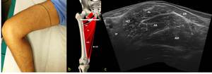
 correlated to EFV US axial scan (c) at proximal third of the thigh (b) that shows the anatomical relationship among the ileopsoas (IP), pectineus (PET), adductor longus (AL), adductor brevis (AB), adductor magnus (AM) and gracilis (GR)muscles. At this level the most superficial muscles are AL and GR; AB lies just deeper to AL; AM appears as a large muscle posterior and deeper to AB. Note the superficial femoral neurovascular bundle.")
Fig. 25:
Anatomical scheme (a) correlated to EFV US axial scan (c) at proximal third of...
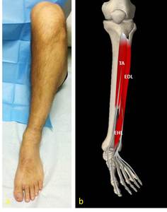
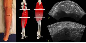
 Leg position to evaluate the anterior leg compartment. (b) Anatomical scheme of anterior leg compartment of extensor muscles : TA, tibialis anterior; EDL, extensor digitorum longus; EHL, extensor hallucis longus. EHL lies in a deeper layer than TA and EDL and its muscle belly arise more distally.")
Fig. 27:
a) Leg position to evaluate the anterior leg compartment. (b) Anatomical scheme...
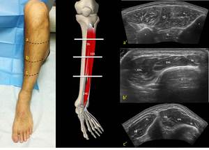
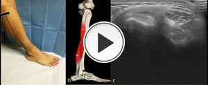
 Proximal third. EFV axial scan visualizes the relationship among the peroneus muscles (P) and the extensor muscles. Tibialis anterior (TA) lies just lateral to tibial crest and medial to Extensor digitorum longus (EDL). The interosseus membrane appears as a hyperechoic well definite layer which separate TA from tibialis posterior muscle (TP). T, tibia; F, fibula. (b, b’) Middle third of anterior compartment. EFV axial scan shows TA myotendinous junction with its oval tendon anterior to tibial edge (T). Note the EDL and EHL muscle bellies.(c, c’) Distal third of anterior compartment. EFV US axial scan evaluates the relationship among the peroneus muscles and the extensor muscles at distal third of leg. Peroneus brevis (PB) and Peroneus longus (PL) are not well separated.")
Fig. 28:
Anatomical scheme correlated to EFV US axial scans at different levels of the...

Fig. 29:
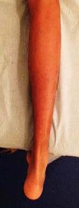
Leg position to evaluate the posterior superficial leg compartment.
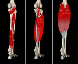
 Deep posterior leg compartment. PO, popliteus, TP, tibialis posterior; FLD, flexor digitorum longus; FLH, flexor halluces longus. TP is deeper than FLH e FDL.(b,c) Superficial posterior leg compartment : Soleus muscle (SO) lies deep to medial and lateral head of Gastrocnemius (GMH, GLH). SO and GMH e GHL insert on distal aponeurosis (SO aponeurosis *; G aponeurosis **) which continues in Achille’s tendon. Fibres from ** form the superficial layer of Achille’s tendon. Plantaris (PL).")
Fig. 30:
Anatomical scheme of posterior leg compartment muscles. (a) Deep posterior leg...
 Proximal third. EFV axial scan visualizes the medial and lateral head of Gastrocnemius which come together in the middle line. Soleus muscle (SO) is deeper than gastrocnemius and is separated from GMH by the distal aponeurosis of G and SO. PO, popliteus muscle. (b, b’) Middle third of superficial posterior compartment. EFV axial scan shows GMH larger than GLH. Distal aponeurosis appears as a hyperechoic band which separates G from SO. At this level note the characteristic internal structure of GLH and GMH consisting of muscular fibres separated by hyperechoic fibroadipose septa.")
Fig. 31:
Anatomical scheme correlated to EFV US axial scans at different levels of the...
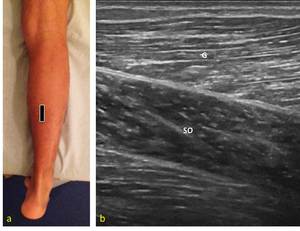
 Probe position to evaluate medial head of gastrocnemius (G) and soleus muscle (SO) on the longitudinal plane. (b) US longitudinal scan : note the distal aponeurosis which appears as a hyperechoic band and separates the two muscles.")
Fig. 32:
(a) Probe position to evaluate medial head of gastrocnemius (G) and soleus...
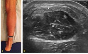
 Probe position to evaluate Achille’s tendon at level of myotendinous junction with an axial plane.(b) US axial scan : at middle of myotendinous junction, Achilles’s tendon (*) originates from distal aponeurosis of soleus (SO) and it is composed of tendinous fibres of gastrocnemius lateral and medial head. Note the fibrillar echostructure and the crescent shape of Achille’s tendon.")
Fig. 33:
(a) Probe position to evaluate Achille’s tendon at level of myotendinous...
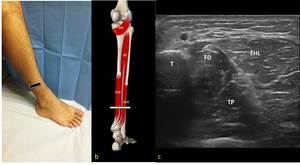
 Probe position to evaluate the flexor muscles at distal leg level on the axial plane. (b) Anatomical scheme of deep posterior compartment. Po, popliteus; TP, tibialis posterior; FDL, flexor digitorum longus; FHL, flexor halluces longus. (c) US axial scan explains the relationship of flexor muscles. TP is deeper than FD and FHL; FHL is the most lateral.")
Fig. 34:
(a) Probe position to evaluate the flexor muscles at distal leg level on the...

Fig. 35:
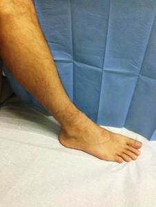
Leg position to evaluate the lateral leg compartment.
 lies superficial to peroneus brevis (PB) and its tendon courses lateral to PB tendon.")
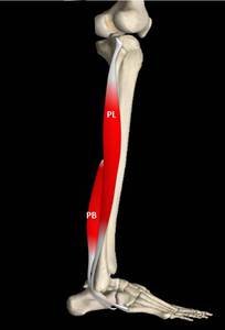
Fig. 36:
Anatomical scheme of lateral leg compartment muscles : peroneus longus (PL)...

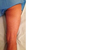
Fig. 15:
Lower limb position to evaluate the posterior thigh compartment.
 to evaluate the medial thigh compartment.")
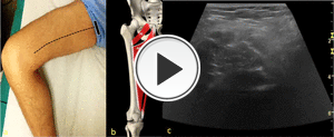
Fig. 21:
Lower limb position (frog leg position) to evaluate the medial thigh...

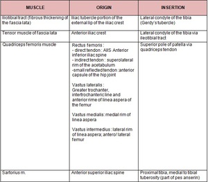
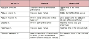
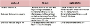
Table 1:
Origin and insertion of the muscles of anterior thigh compartment.

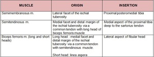
Table 2:
Origin and insertion of the muscles of posterior thigh compartment.

Table 3:
Origin and insertion of the muscles of medial thigh compartment.

Table 4:
Origin and insertion of the muscles of anterior leg compartment.

Table 5:
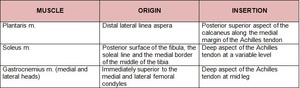
Origin and insertion of the muscles of superficial posterior leg compartment.

Table 6:
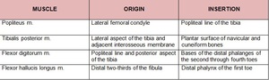
Origin and insertion of the muscles of deep posterior leg compartment.

Table 7:
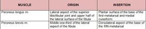
Origin and insertion of the muscles of lateral leg compartment.