Here we present the most useful radiographic measurements for the lower limb,
more specifically for the hip,
knee,
ankle and foot joints.
We will provide clear depiction of the correct application of these measurements.
· FULL-LENGHT LOWER LIMB
1.
Mechanical and anatomical axis of the lower limb
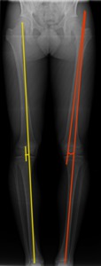
Fig. 1: Normal lower limb alignment: Mechanical axis deviation (yellow) of 13 mm (medial). Anatomical axis angle (red): a non-pathological value of 2º is seen here.
|
Projection(s)
|
Anteroposterior lower limbs full-length standing radiograph
|
| Purpose |
Evaluate the alignment of the lower limbs
|
| Technique |
The mechanical axis (Fig. 1) passes through the center of the femoral head and through the center of the ankle joint (midpoint of the tibial plafond).
The normal mechanical axis should pass just medial to the center point of the knee joint.
The anatomic axis is defined by the axis of the femoral and tibial shafts (Fig.
1).
|
| Criteria |
The mechanical axis deviation (MAD) should be of 10 mm ± 7 mm.
Genu valgum can be diagnosed when MAD is laterally deviated for > 3 mm (normal - SD); Genu varum is considered when MAD is medially deviated for > 17 mm (normal + SD).
[1]
The anatomical tibiofemoral angle is of 6.85º ± 1.4º.
Genu valgum is considered when the angle is higher than 8.3º and genu varum when it is lower than 0º.
[2,
3]
|
Comments
|
The most important image quality criterion for these measurements is to have the patellae centered between the femoral condyles.
|
2.
Limb length
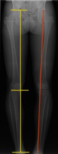
Fig. 2: Femoral and tibial lengths are seen here in yellow. Total limb length measurement shown in red.
| Projection(s) |
Anteroposterior lower limbs full-length standing radiograph
|
| Purpose |
Evaluate lower limb length (relative and absolute).
|
| Technique |
First draw an horizontal line tangent to the superior margin of the femoral head and then measure the length of the femur between that point and the horizontal tangent to the most distal point of the medial femoral condyle.
Tibial length is measured from the later tangent to the horizontal tangent through center of the tibial plafond (Fig. 2).
Total limb length can be determined by measuring the total length from the superior border of the femoral head to the center of the tibial plafond (Fig. 2).
[2,
3,
4]
|
| Criteria |
Bilateral simmetry.
[4]
|
| Comments |
|
· HIP
1.
Projected Neck-Shaft Angle
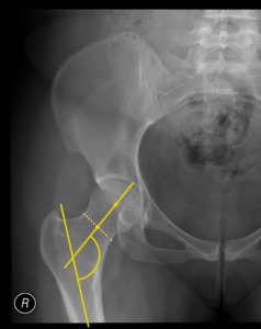
Fig. 3: Normal Neck-Shaft Angle (NSA) of 122º.
| Projection(s) |
Anteroposterior pelvic or hip+femur radiograph.
|
| Purpose |
Evaluate hip alignment.
|
| Technique |
It is the angle formed by the longitudinal axes of the neck and shaft of the femur (Fig. 3).
|
| Criteria |
Normal values in adults are between 120º and 130º; Coxa valga is defined as NSA > 130º,
anda coxa vara as NSA < 120º.[5,
6]
|
| Comments |
Also known as the caput-collum-diaphyseal (CCD) angle.
|
2.
Distance between Anterior and Posterior Acetabular Rims
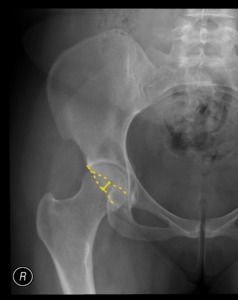
Fig. 4: Normal distance between anterior and posterior acetabular rims (13 mm).
|
Projection(s)
|
Anteroposterior pelvic view
|
| Purpose |
Determine if the acetabulum has a normal or abnormal degree of anteversion.
|
| Technique |
A perpendicular line is drawn from the center of the femoral head to the acetabular rims,
and the distance between the anterior and posterior rims is measured (Fig. 4).
The rims of the acetabulum are not parallel,
making this value only an approximation.
|
| Criteria |
A normal value of 1,5cm is considered.
Higher or lower values are suggestive of increased and decreased anteversion respectively.
[5,
6]
|
Comments
|
Some degree of acetabular anteversion is present in a normal hip.
The distance between the anterior and posterior acetabular rims serves as a simple way of evaluating acetabular anteversion.
|
3.
Acetabular depth
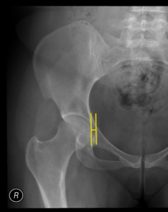
Fig. 5: Male with coxa profunda (acetabular depth is of 6 mm).
|
Projection(s)
|
Anteroposterior pelvic view.
|
| Purpose |
Assess the presence of coxa profunda (a condition in which the acetabular fossa is too deep)
|
| Technique |
Calculate the distance between the medial acetabular roof line and the ilioischial line (Fig. 5).
|
| Criteria |
Coxa profunda is considered critical when the acetabular depth is <-3 mm on men and < -6 mm on women.
[6,
8]
|
Comments
|
|
4.
The Acetabular Index,
the accessory lines of Hilgenreiner and Perkins-Ombredanne,
and the arcs of Shenton-Ménard and Calvé
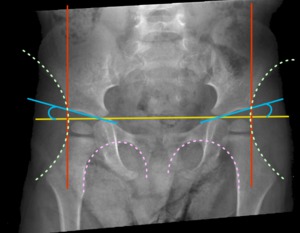
Fig. 6: Bilateral normal hips of a 3 year old infant, with Acetabular Index (blue) of 16º (right) and 13º (left), the accessory lines of Hilgenreiner (yellow) and Perkins-Ombredanne (red) form 4 quadrants (femoral ossification center normally positioned in the infero-medial one), and the arcs of Shenton-Ménard (pink) and Calvé (green) are smooth and uniform.
|
Projection(s)
|
Anteroposterior pelvic view.
|
| Purpose |
Screening of Developmental Dysplasia of the Hip (DDH).
|
| Technique |
Hilgenreiner line: horizontal line drawn across the lowest points of both iliac wings,
tangent to the inferolateral edge of the ilium above the triradiate cartilage.
(Fig. 6)
Perkins-Ombredanne line: perpendicular to the Hilgenreiner line and passes through the most lateral point of the acetabular roof.
(Fig. 6) When drawn alongside the Hilgenreiner line 4 quadrants are defined for each hip joint.(Fig. 6)
Acetabular Index: angle formed by the Hilgenreiner line and a line tangent to the acetabular roof.
(Fig. 6)
Shenton-Ménard arc: curved lined drawn along the medial aspect of the femoral neck and the superior border of the obturator foramen.(Fig. 6)
Calvé arc: arc traced along the lateral border of the iliac wing,
through the superior acetabular rim and the femoral neck.(Fig. 6)
|
| Criteria |
Perkins-Ombredanne quadrants: The femoral ossification center should be below the Hilgenreiner line and medial to the Perkins-Ombredanne line (i.e.
in the infero-medial quadrant).
If the femoral ossification center is located in any of the other 3 quadrants hip dislocation is present.
[2,
3,
8]
Acetabular Index (AI): The normal (mean) AI is age-dependent,
and should be checked on percentile curves or tables (outside the scope of this poster). The diagnosis of DDH is made when the acetabular index is equal or higher than the mean AI plus one standard deviation. One can further subdivide DDH in mild dysplasia (mean+SD ≤ AI < mean+2 SD) and severe dysplasia (AI > mean+2SD).
[2,
3,
8]
Shenton-Ménard and Calvé arcs: If these arcs are not smooth and uniform,
and there is a break or bulge in the line,
the hip is considered dislocated.
[2,
3,
8]
|
Comments
|
In children up to 4 years of age the Acetabular Index is the most important parameter, for the evaluation of older patients the Center-edge (CE) angle of Wiberg and the VCA angle of Lequesne and De Séze are more useful (see below).
|
5.
Center-edge (CE) Angle of Wiberg
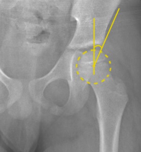
Fig. 7: 6 years old infant, successfully treated for DDH in the past, presenting a normal Center-Edge (CE) angle of Wiberg of 24º.
|
Projection(s)
|
Anteroposterior pelvic view.
|
| Purpose |
Evaluating residual hip dysplasia in children and adults.
|
| Technique |
Angle formed between a line parallel to the longitudinal body-axis and a line connecting the center of the femoral head to the outer edge of the superior acetabular rim (Fig. 7).
|
| Criteria |
Normal values are higher than 20º between ages 5 through 8 and above 25º from 9 years on.
Lower values are diagnostic for hip dysplasia.
[7]
|
Comments
|
The CE is the principal angle for evaluating residual hip dysplasia in children and adults.
[3]
|
6. Tönnis angle
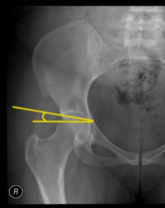
Fig. 8: Normal Tönnis angle of 5º.
|
Projection(s)
|
Anteroposterior pelvic view.
|
| Purpose |
Gauge the slope of the weight-bearing surface of the acetabular roof.
Giving an indirect measure of femoral incongruence (and therefor of stress on the cartilages).
|
| Technique |
A line is traced tangent to the acetabular roof,
passing through the most lateral and inferior points of the weight-bearing (sclerotic) zone.
Then an horizontal line is drawn through the lowest point of both sclerotic zones. The angle formed between the two lines is the Tönnis angle.(Fig. 8)
|
| Criteria |
Normal: 0-10º
< 0º: acetabular overcoverage
>10º: hip dysplasia
|
Comments
|
Also known as the Horizontal Toit Externe (HTE) angle and as the Acetabular Index of the Weight-Bearing Zone.
|
7.
VCA angle of Lequesne and De Séze
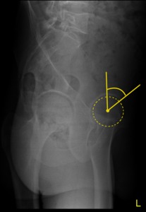
Fig. 9: Normal VCA angle of Lequesne and Séze (44º).
| Projection(s) |
False profile view of the hip ("Lequesne view").
|
| Purpose |
Evaluate the anterior coverage of the femoral head by the acetabulum.
|
| Technique |
Angle formed between a vertical line parallel to the longitudinal body axis which passes through the center of the femoral head and an oblique line traced from the femoral head center to the anterior rim of the acetabulum.
(Fig. 9)
|
| Criteria |
• Normal values: > 25º
• Borderline: 20-25º
• Dysplasia: < 20º [9]
|
| Comments |
|
8.
Epiphyseal slip angle (Southwick method)
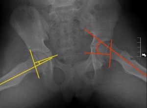
Fig. 10: 12 years old infant with SCFE on the left hip. A normal epyphiseal slip angle (Southwick method) is seen on the right (yellow), and an abnormal value of 33º is present on the left (red).
| Projection(s) |
frog-leg lateral view.
|
| Purpose |
Evaluate Slipped Capital Femoral Epiphysis (SCFE).
|
| Technique |
The epiphyseal baseline is drawn through the corners of the epiphysis,
and the slip angle is formed by a line perpendicular to the epiphyseal baseline (in this view it is the epiphyseal axis) and the femoral shaft axis (Fig. 10).
|
| Criteria |
• mild slip: < 30°
• moderate slip: 30-50°
• severe slip: > 50° [11]
|
| Comments |
Recent discoveries on femoroacetabular impingement have made many authors recommend more rigorous tolerance limits (rather than the 30º cutoff) and expand the indications for surgical intervention.
|
9.
Alpha Angle
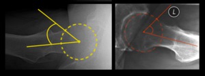
Fig. 11: Normal hip on the right with an alfa angle (yellow) of 34º. Cam femoroacetabular impingement on the left, with a resulting abnormal alfa angle (red) of 60º.
| Projection(s) |
Cross-table lateral view of the hip.
|
| Purpose |
Quantitative measure of the anterior femoral head-neck junction shape in the evaluation of femoroacetabular impingement.
|
| Technique |
The alpha angle is formed between the femoral neck axis and a line traced from the center of the femoral head to the point where the head first becomes aspherical.(Fig. 11)
|
| Criteria |
Normal: <55º
Femoroacetabular Impingement: ≥55º [12,
13]
|
| Comments |
Nowadays the alpha angle is more correctly determined using MRI.
|
10.
Femoral Head-Neck Offset
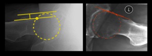
Fig. 12: Normal femoral head-neck offset on the left (yellow) of 12 mm seen on a normal hip, and an abnormal femoral head-neck offset on the right (red) of almost 0 mm seen in a patient with cam femoroacetabular impingement.
| Projection(s) |
Cross-table lateral view of the hip.
|
| Purpose |
Evaluation of femoroacetabular impingement (FAI).
|
| Technique |
The femoral head-neck offset is defined as the distance between two horizontal lines: The first one tangent to the anterior femoral head contour,
and the second one drawn through the point where the head-neck contour leaves the spherical part of the femoral head.
(Fig. 12)
|
| Criteria |
Offset: [12,
13]
• Normal value: 11.6 mm ± 0.17 mm
• Indicator of FAI:<10 mm
Offset ratio (ratio of anterior femoral head-neck offset to femoral head diameter): [3,
12,
13]
• Normal value: 0.21 ± 0.03
• Indicator of FAI: < 0.18
|
| Comments |
|
· KNEE
1.
Insall-Salvati Index
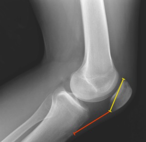
Fig. 13: Normal height patella. Patellar diagonal length (yellow) of 53 mm and patellar tendon length (red) of 65 mm. The Insall-Salvati Index is 0,82 (53/65).
| Projection(s) |
Lateral knee view (with 20º-70º flexion).
|
| Purpose |
Diagnosing patella alta.
|
| Technique |
The greatest diagonal length of the patella is measured from its posterosuperior corner to the apex.
The length of the patellar tendon is measured from the patellar apex to the tibial tuberosity.
The ratio of these two measurements is the Insall-Salvati index. (Fig. 13)
|
| Criteria |
• Normal range: 0.8-1.2
• High-riding patella (patella alta): < 0.8
• Low-riding patella (patella infera): > 1.2 [14]
|
| Comments |
|
2.
Sulcus angle
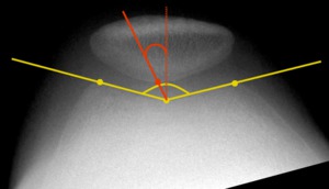
Fig. 14: Slight trochlear displasya. Sulcus angle (yellow) of 151º and patellofemoral congruence angle (red) of 53º.
| Projection(s) |
Knee tangential view ("sunrise").
|
| Purpose |
Assessing trochlear dysplasia.
|
| Technique |
The lines forming the angle are obtained by tracing through the deepest point of the trochlea and the highest points on the medial and lateral femoral condyles.
(Fig. 14)
|
| Criteria |
• Normal range: ≤145º
• Trochlear dysplasia: >145º [15,
16]
|
| Comments |
Also known as the β (beta) angle and as the throclear angle.
|
3.
Patellofemoral congruence angle
| Projection(s) |
Knee tangential view ("sunrise").
|
| Purpose |
Evaluating patellofemoral joint congruence.
|
| Technique |
The patellofemoral congruence angle is defined as the angle formed between the bisector of the sulcus angle (see above) and a line traced through the deepest point of the trochlea and the lowest point of the pattelar ridge. (Fig. 14)
|
| Criteria |
• Mean Value: -6º±11º
• Abnormal: > 16º [15,
16]
|
| Comments |
|
4.
Axial linear Patellar Displacement
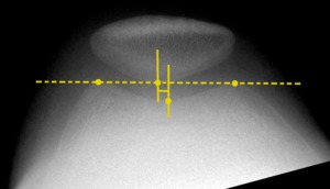
Fig. 15: Normal Axial linear Patellar Displacement (on a right knee) of -4mm (medial).
| Projection(s) |
Knee tangential view ("sunrise").
|
| Purpose |
Evaluating patellofemoral joint congruence.
|
| Technique |
First a line passing through the highest points on the medial and lateral femoral condyles is defined.
Then two perpendicular lines are drawn from that line: one through the deepest point of the trochlear sulcus and one through the lowest point on the patellar ridge.
The distance between the two perpendicular lines constitutes the axial linear patellar displacement.
(Fig. 15)
|
| Criteria |
• Normal range: ≤ 2 mm
• Abnormal lateralization: > 2 mm [17,
18]
|
| Comments |
|
5.
Lateral patellofemoral angle of Laurin
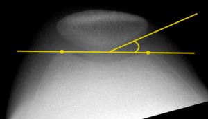
Fig. 16: Normal (acute on the lateral side) lateral Patellofemoral Angle of Laurin.
| Projection(s) |
Knee tangential view ("sunrise").
|
| Purpose |
Screening recurrent patellar subluxation.
|
| Technique |
The Laurin angle is formed between a line tangent to the
highest points on the medial and lateral femoral condyles and a line across the lateral patellar facet.
( Fig. 16 )
|
| Criteria |
• Normal joint: acute angle formed on the lateral side
• Patellar Instability: acute angle formed on the medial side (or parallel lines).
[16]
|
| Comments |
|
· ANKLE AND FOOT
1.
Calcaneal Inclination Angle
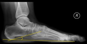
Fig. 17: Slightly planovalgus foot, with a calcaneal inclination angle of 17º.
| Projection(s) |
Standing lateral view of the foot.
|
| Purpose |
Assessing deformities of the longitudinal arch of the foot.
|
| Technique |
Angle formed by a line tangent to the inferior cortex of the calcaneus and an horizontal reference line (or the plantar
plane).
(Fig. 17)
|
| Criteria |
• Normal range: 20-30º
• Flatfoot (pes planovalgus): < 20º
• Pes cavus: > 30º [18,
19]
|
| Comments |
|
2.
Talar Declination Angle
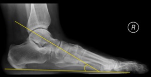
Fig. 18: Normal talar declination angle (28 º).
| Projection(s) |
Standing lateral view of the foot.
|
| Purpose |
Assessing deformities of the longitudinal arch of the foot.
|
| Technique |
Angle defined by the longitudinal axis of the talus and a horizontal reference line (or the plantar plane). (Fig. 18)
|
| Criteria |
• Normal range: 14-35º
• Flatfoot (pes planovalgus): > 35º
• Pes cavus: < 14º [18,
19]
|
| Comments |
|
3.
Talar-First Metatarsal Angle
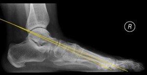
Fig. 19: Normal talar-first metatarsal angle (of aprox. +4º).
| Projection(s) |
Standing lateral view of the foot.
|
| Purpose |
Assessing deformities of the longitudinal arch of the foot.
|
| Technique |
Angle formed between the longitudinal axis of the first metatarsal shaft and the longitudinal axis of the talus. (Fig. 19)
|
| Criteria |
• Normal range: -4º to +4º
• Flatfoot (pes planovalgus): < -4º
• Pes cavus: > 4º [18,
19]
|
| Comments |
In a normal pedal arch,
the two axes are parallel or congruent so that the talar-first metatarsal angle is around 0º.
|
4.
Böhler Angle
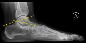
Fig. 20: Normal Böhler angle (30º).
| Projection(s) |
Lateral ankle (or foot) view.
|
| Purpose |
Evaluate calcaneal deformity resulting from fracture.
|
| Technique |
Angle formed by the lines tangent to the posterosuperior and anterosuperior borders of the calcaneus. (Fig. 20)
|
| Criteria |
Normal range: 20-40º [18-20]
|
| Comments |
Also written as Bohler angle or Boehler angle.
Also known as the Tuber Joint Angle.
With fractures involving the anterior process of the calcaneus,
the angle is decreased and may present negative values.
|
5.
Talocalcaneal angle (lateral and dorsoplantar)
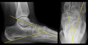
Fig. 21: Adult with normal talocalcaneal angle, of 46º and 25º as measured on lateral (left) and dorsoplantar (right) views respectively.
| Projection(s) |
Lateral and dorsoplantar foot views.
|
| Purpose |
Indicator of hindfoot alignment.
|
| Technique |
Lateral view: formed by the longitudinal axis of the talus and a tangent to the inferior calcaneal border (equals the longitudinal calcaneus axis). (Fig. 21)
Dorsoplantar view: formed by the longitudinal axes of the talus and the calcaneus. (Fig. 21)
|
| Criteria |
Lateral view [20-23]
• Normal range:
- Newborns: 25-55º
- Adults: 30-50º
• Hindfoot valgus: > 55º
• Hinfdoot varus: < 30º
Dorsoplantar view [20-23]
• Normal range:
- Newborns: 25-55º
- Adults: 20-45º
• Hindfoot valgus: > 45º
• Hinfdoot varus: < 20º
|
| Comments |
The talocalcaneal angles are important in the diagnosis of congenital foot deformities in clubfoot.
|
6.
Metatarsal Index
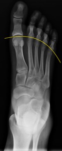
Fig. 22: Example of a plus-minus index (the distal end of the first metatarsal head touches the arc).
| Projection(s) |
Dorsoplantar foot view.
|
| Purpose |
Estimation of the length relationship between the first and the remaining metatarsals.
|
| Technique |
Drawing an uniform arc across the distal ends of the second through fifth metatarsals. (Fig. 22)
|
| Criteria |
• Plus index: The head of the first metatarsal is distal to the arc.
• Plus-minus index: Distal end of the first metatarsal head touches the arc.
• Minus index: The first metatarsal head is proximal to the arc.
[23]
|
| Comments |
A minus index indicates predisposition to hallux valgus and (associated) metatarsalgia due to increased loads on the second and third metatarsal heads.
From a therapeutic perspective,
hallux valgus deformities with a minus index of the metatarsals should not be treated with osteotomy that shortens the first metatarsal.
|
7.
Tarsal joint surface angles
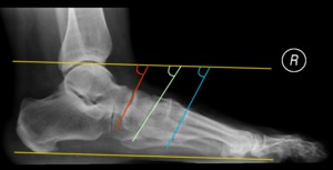
Fig. 23: Normal tarsal joint surface angles: Talonavicular surface angle (red) of 64º; Naviculocuneiform surface angle (green) of 61º and first tarsometatarsal surface angle (blue) of 64º.
| Projection(s) |
Lateral foot view.
|
| Purpose |
Evaluation of the alignment of the tarsal joints.
|
| Technique |
The angles are formed by a line parallel to the plantar plane and straight lines drawn through the tarsal articular surfaces (talonavicular,
naviculocuneiform and first tarsometatarsal).
(Fig. 23)
|
| Criteria |
• Talonavicular joint: 54-74º
• Naviculocuneiform joint: 51-68º
• First tarsometatarsal joint: 55-72º [2,
20-23]
|
| Comments |
|
8.
First-Fifth intermetatarsal angle
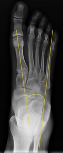
Fig. 24: Normal first-fifth intermetatarsal angle of 15º.
| Projection(s) |
Dorsoplantar foot view.
|
| Purpose |
Screening for abnormal widening of the forefoot (pes transversus - splayfoot).
|
| Technique |
Angle formed between the longitudinal axes of the first and fifth metatarsals. (Fig. 24)
|
| Criteria |
• Normal range: 14-35º
• Splayfoot (pes transversus): > 35º [2,
3,
21]
|
| Comments |
Pes transversus can be the cause for secondarily development of hallux valgus as well as lesser toe deformities.
|
9.
Hallux Valgus Angle
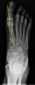
Fig. 25: Normal first metatarsal-proximal phalanx angle of 9º (no evidence of hallux valgus).
| Projection(s) |
Dorsoplantar foot view.
|
| Purpose |
Evaluating hallux valgus (lateral deviation of the first toe).
|
| Technique |
Angle formed by the longitudinal axes of the first metatarsal and first proximal phalanx. (Fig. 25)
|
| Criteria |
• Normal value: ≤ 15º
• Hallux valgus: > 15º [20]
|
| Comments |
|
10.
Simplified metatarsus adductus angle (Engel Method)
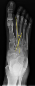
Fig. 26: Simplified metatarsus adductus angle (Engel method), with a normal 20º value (without metatarsus adductus).
| Projection(s) |
Dorsoplantar foot view.
|
| Purpose |
Grading the medial deviation of the forefoot at the Lisfranc joint.
|
| Technique |
Angle formed by the longitudinal axis of the lesser tarsus (represented on the simplified Engel method by the longitudinal axis of the medial cuneiform) and the longitudinal axis of the second metatarsal. (Fig. 26)
|
| Criteria |
• Normal range: 13-23º
• Metatarsus adductus: > 23º [24]
|
| Comments |
The metatarsus adductus angle is only useful in children whose tarsal bones are mostly ossified and have well defined margins.
In newborns and small children,
the angle between the longitudinal axis of the calcaneus and the second metatarsal is preferred for the evaluation of the relationship of the tarsus and metatarsals.
|
11.
Plantar soft-tissue thickness
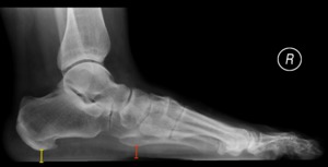
Fig. 27: Normal plantar soft-tissue thickness (8 mm in both calcaneal and metatarsal evaluation sites).
| Projection(s) |
Lateral foot view.
|
| Purpose |
Diagnosing thickening of the plantar fat pad.
|
| Technique |
The thickness of the plantar soft tissues is measured as the distance between the skin line and both the lowest point of the calcaneus and the inferior margin of the proximal fifth metatarsal head. (Fig. 27)
|
| Criteria |
• Normal values: [25]
- Calcaneal fat pad: ≤ 25 mm
- Metatarsal fat pad: 5-16 mm
• Values in acromegaly: [25]
- Calcaneal fat pad: > 25 mm
- Metatarsal fat pad: > 16 mm
|
| Comments |
Although a hallmark of acromegaly, thickening of the plantar fat pad may occur in other diseases (myxedema,
reflex sympathetic dystrophy,
lymphedema,
traumatic edema).
|
12.
Philip-Fowler angle
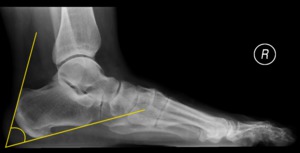
Fig. 28: Normal Philip-Fowler angle (60º).
| Projection(s) |
Lateral foot view.
|
| Purpose |
Measuring Haglund deformity (abnormal prominence/projection of the posterosuperior calcaneus).
|
| Technique |
Angle formed between a line tangent to the posterosuperior border of the calcaneus and the calcaneal tuberosity and a line tangent to the inferior border of the calcaneus (longitudinal axis of the calcaneus). (Fig. 28)
|
| Criteria |
• Normal range: 44-69º
• Prominence of superior calcaneal tuberosity: > 75 º [26]
|
| Comments |
|

 of 13 mm (medial). Anatomical axis angle (red): a non-pathological value of 2º is seen here.")

 of 122º.")
.")
.")
 of 16º (right) and 13º (left), the accessory lines of Hilgenreiner (yellow) and Perkins-Ombredanne (red) form 4 quadrants (femoral ossification center normally positioned in the infero-medial one), and the arcs of Shenton-Ménard (pink) and Calvé (green) are smooth and uniform.")
 angle of Wiberg of 24º.")

.")
 of 34º. Cam femoroacetabular impingement on the left, with a resulting abnormal alfa angle (red) of 60º.")
 of 12 mm seen on a normal hip, and an abnormal femoral head-neck offset on the right (red) of almost 0 mm seen in a patient with cam femoroacetabular impingement.")
 of 53 mm and patellar tendon length (red) of 65 mm. The Insall-Salvati Index is 0,82 (53/65).")
 of 151º and patellofemoral congruence angle (red) of 53º.")
 of -4mm (medial).")
 lateral Patellofemoral Angle of Laurin.")

.")
.")
.")
 and dorsoplantar (right) views respectively.")
.")
 of 64º; Naviculocuneiform surface angle (green) of 61º and first tarsometatarsal surface angle (blue) of 64º.")
.")
, with a normal 20º value (without metatarsus adductus).")
.")
.")
 is seen on the right (yellow), and an abnormal value of 33º is present on the left (red).")