A CT equipment
For the measurements, a multi-axis C-arm Artis prototype (Siemens Healthcare, Forchheim, Germany) has been used. It is equipped with a large flat-panel detector of 40.0 x 30.0 cm² size.
B Reconstruction platform
- Modular design.
- Standard Feldkamp (FDK) algorithm.
- Process flat-detector raw-data formats from various FD-CT manufacturers.
- Partial scan reconstruction (Parker weighting) that needs only a scan over 180° plus fan-angle.
- Real-to-ideal geometry rebinning to ensure the portability between different FD-systems.
- Analytic water precorrection (beam-hardening correction).
- Convolution with various selectable kernels.
- Up to 1024³ voxels volume reconstruction.
- Isotropic resolution of 0.1 - 0.3 mm [1].
- Multiplanar reformations (MPR).
- Advanced correction steps explained below.
C Misalignment correction Misalignment signifies the deviation between ideal (expected) and real geometry. Due to mechanical instabilities, C-arm CT systems are prone to misalignment and thus, misalignment calibration becomes necessary.
For misalignment correction, a calibration phantom that contains steel spheres with known positions is regularly scanned. The steel spheres are segmented in the single projections and thus the misalignment parameters ξ are determined for each projection [2].
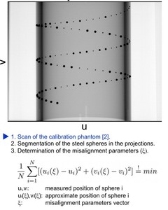
Fig.: The known location of the steel spheres within the phantom is used to determine the misalignment parameters for each projection.
Fig.: This animated GIF explains the misalignment correction using a special phantom for calibration.
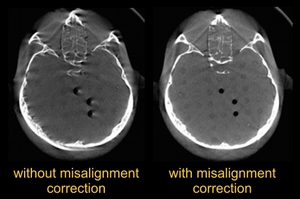
Fig.: This image shows a slice of a head phantom with and without misalignment correction.
D Detruncation
Due to the limited field of view in FD-CT (about 15 – 25 cm) the volume is not entirely scanned and therefore the sinogram data is incomplete which leads to truncation artifacts.
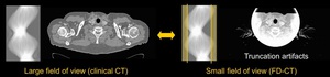
Fig.: In flat-detector CT, truncation artifacts occur for bigger patient sizes due to the limited field of view which leads to incomplete sinogram data.
The individual projections are corrected using extrapolation functions that smoothly decline to zero attenuation at the edge of the extended projection [3] [4]. The reconstruction can be done using either the original field of view or an extended field of view.
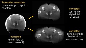
Fig.: This figure shows the results of truncation correction on the measured data of an antropomorphic phantom. For the reconstruction, either the original or an extended field of view may be used.
E Scatter correction
FD-CT provides wide collimation in z-direction which results in increased scatter artifact content. A scatter-to-primary ratio exceeding 1.0 for some detector pixels is not unusual [5].
The implemented scatter correection algorithm is based on physical scatter modelling. Segmentation of a first reconstruction provides estimates for the scatter properties of each voxel. A hybrid method is used in order to optimize the performance of the scatter simulation: a fast and exact analytical calculation of the single-scatter intensity combined with a coarse Monte Carlo (MC) estimate of multiple scatter to reduce overall computational expense, while assuring an acceptable signal quality [5]. For higher image quality, the algorithm can be used iteratively.
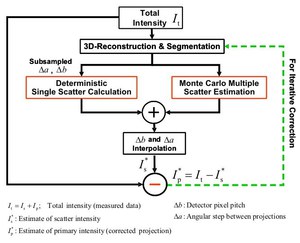
Fig.: This figure explains the developed scatter correction algorithm. It uses a hybrid method combining analytical and Monte Carlo calculations for scatter estimation. To further improve image quality, the algorithm can be used iteratively.
The scatter correction successfully removes cupping artifacts present in uncorrected CT slides.
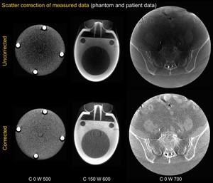
Fig.: This figure shows CT slices of two phantoms and of one patient with and without scatter correction. The scatter correction removes the cupping artifacts.
For simulations, image quality improvement can be quantified by calculating and summing the root mean square distances of the CT value of each voxel in the reconstructed volume compared with the reference image that has been simulated without scatter. A scatter correction quality number of Q = 1.0 is assigned to the reference image and a number of Q = 0.0 is assigned to the uncorrected image. Similar quality numbers can also be applied to other corrections.
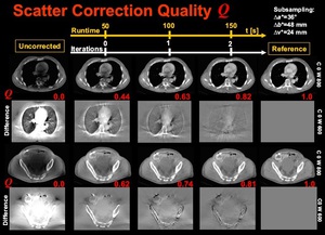
Fig.: A scatter correction quality of Q = 0.0 is assigned to the uncorrected image and a scatter correction quality of Q = 1.0 is assigned to the simulated scatter-free image. The quality improves with iterations. Here, one iteration of the scatter correction algorithm lasted for about 50 s on a standard PC. However, this value depends on subsampling.
F Metal artifact reduction (MAR)
Rays that intersect metal objects are highly attenuated and thus only a low number of photons arrive at the detector which leads to unprecise attenuation coefficients. In the reconstructed image, streak-like artifacts emanate from metallic objects, e.g. dental prostheses or hip implants. This severly deteriorates image quality and increases directional noise.
To reduce metal artifacts, the “metal”-voxels are segmented in the reconstructed volume and forward-projected to the original projections. There, the value is corrected by linear interpolation of the surrounding pixels and the corrected projections are used for further processing.
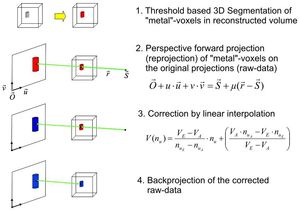
Fig.: This figure explains the algorithm used to reduce metal artifacts.
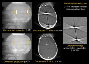
Fig.: This figure compares the reconstruction with and without metal artifact reduction. The measured phantom is a head phantom containing two metal cylinders.
G Multi-dimensional adaptive filtering (MAF)
A low number of photons in directions of high attenuation (photon starvation) causes directional noise artifacts.
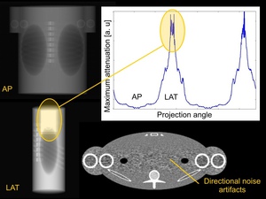
Fig.: This figure explains the occurance of directional noise due to photon starvation. In directions with high attenuation the detector is hit by a low number of photons so that the signal-to-noise increases. This causes directional noise artifacts in the CT slices.
To correct these artifacts, the maximum attenuation pmax is determined throughout an initial range of projection angles, typically 90°. Dependent on the angle of the projection, the projection data p is combined with a low-pass filtered version of the projection pfilt based on the equation
pAF = (1 - wAF) · p + wAF · pfilt.
The weighting factor wAF depends on the maximum attenuation p of the current projection.
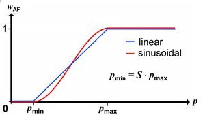
Fig.: The weighting factor depends on the maximum attenuation of the current projection. The lower limit for correction is given by the parameter S. The curce can be linear or sinusoidal.
No correction is done for
p ≤
pmin, maximum correction is done for
p ≥
pmax.
pminis a fixed fraction
S of
pmax,
pmin =S·pmax. The software allows to use both linear and sinusoidal weighting curves.
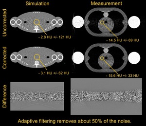
Fig.: This figure shows the results of the adaptive filtering algorithm on a measured and on a simulated phantom. Adaptive filtering removes about 50% of the noise.
Adaptive filtering removes about 50% of the noise σ² or, if the noise is kept constant, the dose D can be reduced according to σ²~1/D.
