Report data: Reports for CT pulmonary embolism examinations from a university hospital was collected (n=22305).
The reports were categorized into five categories by two medical experts.
The experts only had access to the clinical history and the report text,
no images (Fig. 1).
The categories (decided on by the medical experts) were:
-
Embolism (n=3512)
-
No embolism (n=16890)
-
Previously known embolism/No increase (n=160)
-
Uncertain (n=289)
-
Not applicable (n=1454,
these include reports for examinations that had been incorrectly marked as CT pulmonary embolism examinations)
The dataset was split into training/development/test sets (n=14275,
3569,
4461,
respectively).
Preprocessing: We train a logistic regression classifier ([2]) to predict if a report indicates the presence of pulmonary embolism or not.
The classification task is binary,
so the labels given to the reports by the medical experts are folded into two categories,
positive or negative.
Reports labeled with Embolism are considered positive all other reports are considered negative.
The report texts are preprocessed by replacing all numbers by ‘#’ and stemming ([1]) the words using a Swedish stemmer.
The preprocessed texts are then converted into a numerical format by using bag-of-n-grams features (uni- and bi-grams).
Tokens not occurring more than 10 times are removed and only the 3000 most frequent tokens are retained.
Rate prediction: To quantify the rate of positive findings in a set of reports we apply the trained classifier to the preprocessed report texts. This gives us a set of predictions,
D={ûi},
of whether the reports are positive or negative.
We model the predictions as coming from a Bernoulli distribution Û~Be(γ),
where γ is the observed rate of positive findings.
Using a Bayesian approach ([5]) we put a Beta(s,
f)-prior on γ and compute the posterior distribution given the observations ûi.
Fig. 2
As Beta is the conjugate prior to the data likelihood,
the posterior will get the same functional form as the prior with the posterior parameters,
s’=ns+s,
f’=nf+f,
where ns and nf is the number of positive and negative predictions respectively.
From the posterior we calculate a 95% credible interval for γ.
Noisy channel: We relate the observed rate of positive findings to the true rate of positive findings by treating the classifier as a noisy channel ([4]).
The true label of a report,
ui,
is modelled as being drawn from U~Be(θ),
where θ is the true rate of positive findings.
The true label is then fed through the noisy channel (the classifier) and we observe, ûi (Fig. 3).
In this model the observed rate of positive findings,
γ,
can be written:
(Eq.
1)
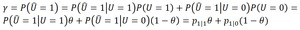
Fig. 4: Eq. 1 Relating the observed rate of positive findings to the true rate of positive findings.
The transition-probabilities p1|1= P(Û=1|U=1),
p1|0= P(Û=1|U=0) can be estimated from the confusion matrix of the classifier.
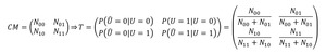
Fig. 6: Estimation of transiton-probabillities from the confusion matrix.
Using Eq.
1 we can translate the credible interval computed from the predictions of the classifier to a credible interval for the true rate of positive findings (we assume p1|1 > p1|0,
which is true for any reasonable classifier):
(Eq.
2)

Fig. 5: Eq. 2 Deriving the relationship between credible intervals on observed and true rates.
From Eq.
2 we can see how the characteristics of the classifier affects the width of the credible interval.
We note that the credible interval for the true rate is always at least as wide as the interval for the observed rate and the less accurate the classifier is (p1|0 approaches p1|1) the wider the true rate credible interval becomes,
which is intuitively pleasing.


