ECR 2014 / C-1988

Analysis of spatial dependence of acoustic noise transfer function in magnetic resonance imaging
This poster is published under an open license. Please read the disclaimer for further details.
Congress:
ECR 2014
Poster Number:
C-1988
Type:
Scientific Exhibit
Keywords:
Safety, MR, MR physics, Quality assurance
Authors:
T. Hamaguchi1, T. Miyati1, T. Matsushita2, N. Ohno1; 1Kanazawa/JP, 2Kyoto/JP
DOI:
10.1594/ecr2014/C-1988
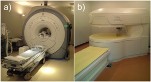
 3.0-T superconducting MRI system (Signa Excite HDxt, General Electric Healthcare, Wisconsin, USA),
b) 0.4-T permanent magnet open MRI system (APERTO Eterna, Hitachi medical corporation, Tokyo, Japan).")
Fig. 2:
a) 3.0-T superconducting MRI system (Signa Excite HDxt, General Electric...
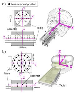
 superconducting MRI system (143 points) and b) permanent magnet open MRI system (75 points).")
Fig. 3:
The measurement positions inside the bore in the a) superconducting MRI system...

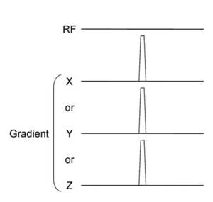
Fig. 4:
Gradient pulse were excited for each gradient.
Pulse sequence was programmed...

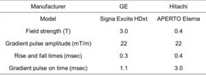
Table 1:
Characteristic of narrow trapezoidal input waveform

Fig. 5:
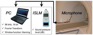
Experimental set-up for acoustic noise measurement.

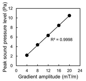
Fig. 6:
Relation between gradient amplitude and acoustic noise.
A strong positive...
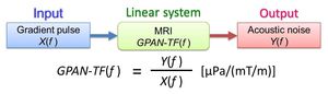
, by the deconvolution process.")
Fig. 7:
Calculation of GPAN-TF in each gradient coil (X, Y, and Z-axis), by the...