ECR 2014 / C-1988

Analysis of spatial dependence of acoustic noise transfer function in magnetic resonance imaging
This poster is published under an open license. Please read the disclaimer for further details.
Congress:
ECR 2014
Poster Number:
C-1988
Type:
Scientific Exhibit
Keywords:
Safety, MR, MR physics, Quality assurance
Authors:
T. Hamaguchi1, T. Miyati1, T. Matsushita2, N. Ohno1; 1Kanazawa/JP, 2Kyoto/JP
DOI:
10.1594/ecr2014/C-1988
.")
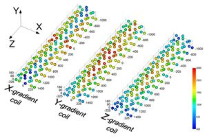
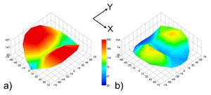
Fig. 8:
Spatial distribution of GPAN-TFs in a superconducting MRI (3.0 T).

Fig. 9:
GPAN-TF of the X coil reached its peak at ±X sides from the isocenter.
 GPAN-TF of the Y coil had a maximum value at a higher position than the isocenter (Z=0).
b) GPAN-TF of the Z coil showed bimodal peaks on the patient axis (Y=0).")
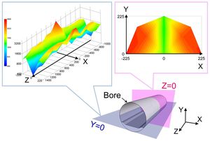
Fig. 10:
a) GPAN-TF of the Y coil had a maximum value at a higher position than the...
.")
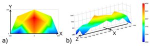
Fig. 11:
Spatial distribution of GPAN-TFs in a permanent magnet open MRI (0.4 T).
 X and b) Y coils were present in ±X and ±Y directions from the isocenter, respectively.")
Fig. 12:
Maximum values of GPAN-TFs for the a) X and b) Y coils were present in ±X and...
 3.0-T superconducting MRI system and b) 0.4-T permanent magnet open MRI system.")
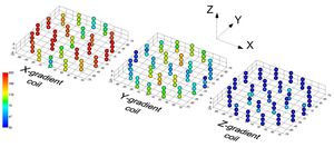
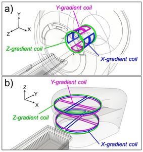
Fig. 13:
Shapes and designs of the gradient coils in the a) 3.0-T superconducting MRI...
 and 0.4-T (right) MRI systems.")
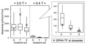
Fig. 14:
Comparison of boxplot distribution for GPAN-TFs at all measurement positions in...
 3.0-T and b) 0.4-T MRI scanner at isocenter.")
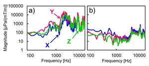
Fig. 15:
Spectra of GPAN-TFs in the a) 3.0-T and b) 0.4-T MRI scanner at isocenter.